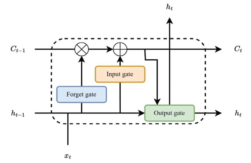
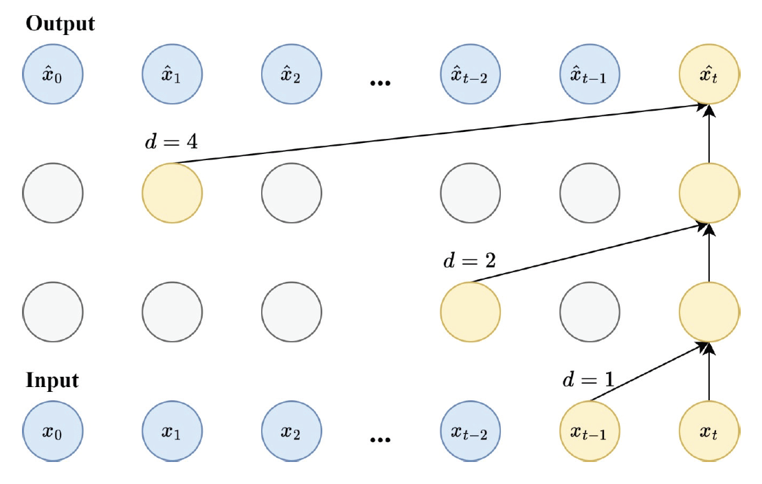
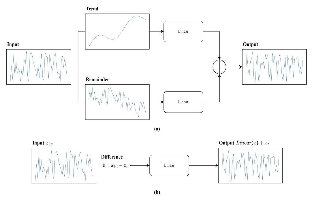
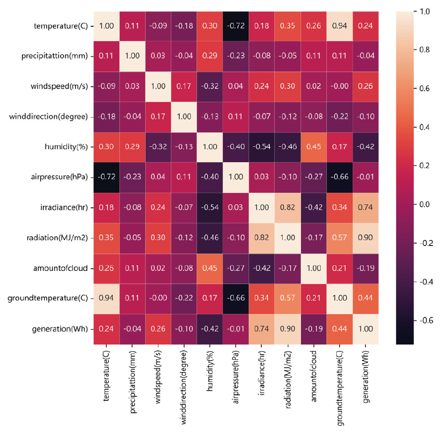
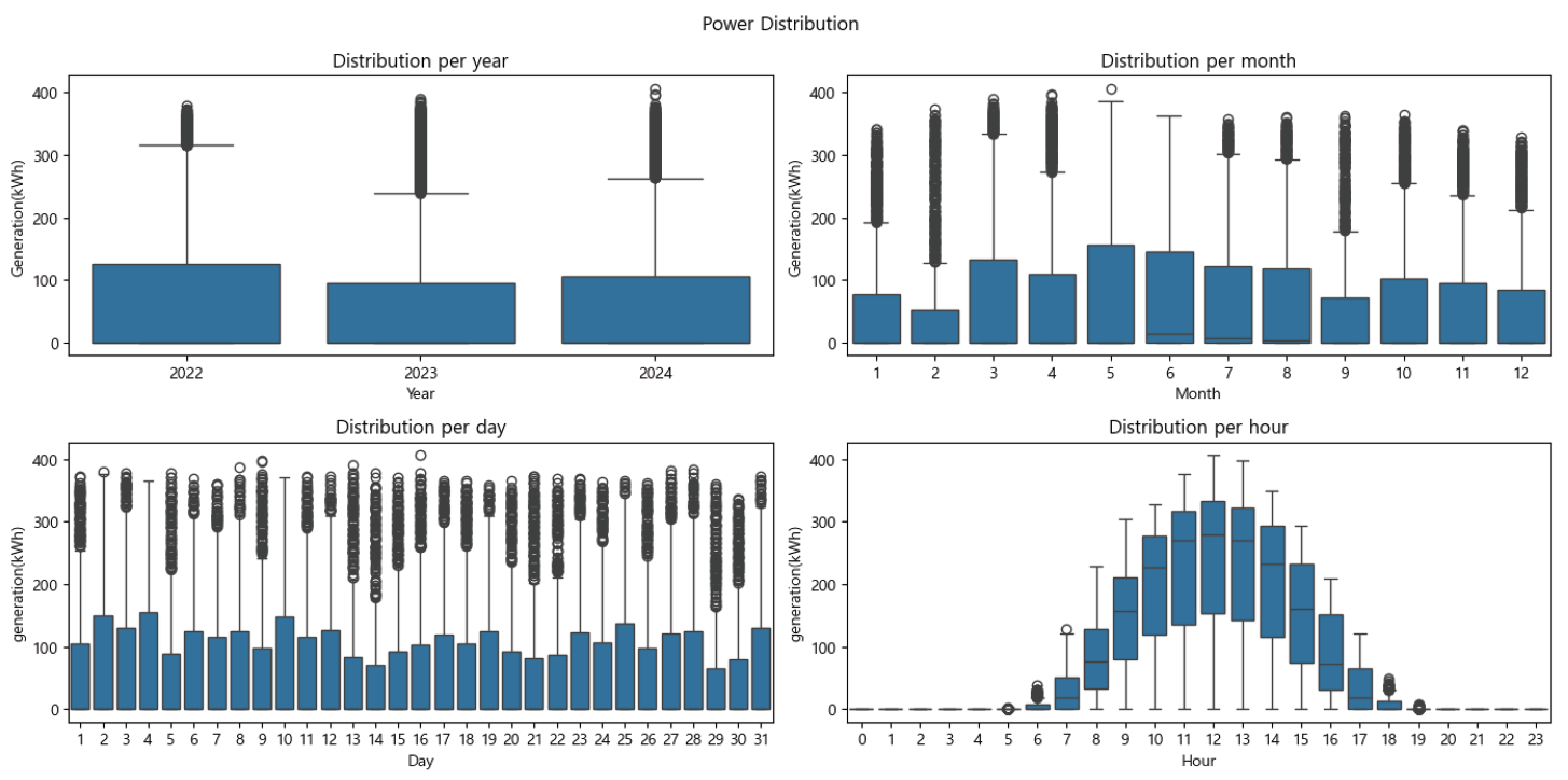
1. Introduction

Climate change and global warming are critical global challenges that demand immediate and innovative solutions. Traditional energy sources such as coal and oil significantly contribute to environmental degradation, emphasizing the urgent need for sustainable energy alternatives. Renewable energy sources, including solar, wind, and water, have emerged as essential components for a sustainable future. Solar energy, in particular, has gained widespread adoption due to its potential for clean and efficient power generation. However, its reliance on external factors such as solar radiation, time of day, and weather conditions introduces variability and unpredictability in power generation, posing challenges for effective integration into the power grid [1]. The International Energy Agency (IEA) estimates that photovoltaic (PV) systems will achieve a peak power capacity of 1200 GW by the end of 2023 [2]. These systems, commonly installed in open areas, on rooftops, and in solar power plants, offer a promising path to reducing dependence on traditional energy sources. Despite their advantages, the intermittent nature of solar power generation disrupts regular operations, complicating energy distribution and grid stability. For instance, fluctuating solar radiation and environmental conditions can lead to energy deficits or surpluses, necessitating advanced forecasting systems to optimize energy storage and usage [3]. Reliable forecasting of solar power generation is essential for ensuring grid stability and maximizing the benefits of renewable energy. Unlike traditional power plants that offer predictable energy outputs, solar energy systems depend on dynamic environmental conditions, making accurate forecasting crucial for energy management. Effective prediction of energy generation enables better planning for storage during surplus periods and ensures energy availability during low-generation intervals [4].

Recent advancements in deep learning have demonstrated significant potential in addressing the challenges of solar power forecasting. Time series forecasting techniques such as Long Short-Term Memory (LSTM) networks, linear models, and attention mechanisms have proven effective in capturing complex patterns and irregularities in solar power data. These approaches surpass traditional methods like physical and statistical models, which often struggle with non-linearities and variability in data [5]. To address these challenges, this study proposes a hybrid deep learning model combining LSTM and linear models with a multi-head attention mechanism. The hybrid model leverages the strengths of each component: LSTM networks capture short-term dependencies and irregular patterns, linear models identify long-term trends, and the multi-head attention mechanism enhances feature extraction by focusing on critical temporal relationships. By integrating these techniques, the proposed model achieves superior forecasting performance, offering a reliable solution for managing the complexities of solar power generation [6]. Extensive experiments conducted in this study demonstrate that the hybrid model outperforms existing forecasting approaches by approximately 10% in prediction accuracy. Additionally, ablation studies validate the effectiveness of integrating multi-head attention with LSTM and linear models, highlighting its ability to capture trends and irregularities in time series data. These findings underscore the potential of the proposed hybrid approach to advance solar energy forecasting and enhance its integration into the energy grid [7-8].

The main contributions of this research work are as follows:

· We propose a novel hybrid model that integrates LSTM networks and linear models with a multi-head attention mechanism to enhance solar power generation forecasting.

· The hybrid model effectively captures both short-term irregularities and long-term trends in time series data, addressing the inherent variability of solar power generation.

· By leveraging the multi-head attention mechanism, the model learns richer temporal features and focuses on critical patterns in historical data for improved prediction accuracy.

· Extensive experiments demonstrate that the proposed hybrid model outperforms existing stateof- the-art prediction methods by approximately 10% in forecasting accuracy.

· Ablation studies validate the effectiveness of combining LSTM, linear models, and attention mechanisms, highlighting the contributions of each component to the overall performance.

The rest of this article is organized as follows: Section 2 reviews the related works, followed by a comprehensive description of background knowledge and the proposed methodology in Sections 3 and 4. Section 5 presents the experimental results and analysis, while Section 6 providing key insights and discusses future directions. Finally, the last section, Section 7 concludes the study.

2. Related Works

With the unpredictability of green energy, e.g. solar power, when compared with energy sources such as nuclear, oil, and coal for example, the need for methods that can forecast the power output becomes clear. As such, this problem has received a lot of attention in recent years, some of which will be introduced in this section.

Prema et al. [9] provide a lot of insight into the field of solar power generation prediction in their review paper, with a focus on datasets, models used, as well as common performance metrics. The paper reviews not only solar power, but also wind power applications. The paper identifies irradiance as the feature with the greatest impact on prediction performance. The authors state that deep learning technologies have shown great results recently, but point out that short-term prediction (up to 1 or 2 days) is recommended. Lastly the study found that the Mean Absolute Error (MAE), Mean Absolute Percentage Error (MAPE), and Symmetric Mean Average Percentage Error (SMAPE) are the most commonly used metrics.

Shin et al. [10] performed solar power generation forecasting using deep learning techniques on a dataset that was collected in Mokpo in Korea. The data was collected over 2 years between 2013 and 2015. The dataset included solar irradiance and solar radiation and the models trained on said data were based on ANFIS, DNN, Recurrent Neural Network (RNN) and LSTM. The authors’ results showcase that the RNN model managed to perform better than the other models used in this work based on the metrics used (RMSE, MAE, BIAS, and COR).

Park et al. [11] analyze the performance of BiLSTM and SHAP-based XAI techniques in solar power forecasting. This work also uses power data obtained in Korea, from different plants across the country. The integration of XAI allows researchers to better understand the trained models and, therefore, also allows them to update the model based on that, overcoming the common “black-box” problem that Deep Learning (DL) models often pose.

Khan et al. [12] incorporated attention mechanisms into their DL model. The dual stream network utilizes both CNN and GRU methods, allowing the model to capture both spatial and temporal relations. This is then combined with a self attention block to further learn relations present in the data. Three datasets were used during the ex periments and MSE, RMSE, a nd MAE i ndicate that t he

2. Related Works

With the unpredictability of green energy, e.g. solar power, when compared with energy sources such as nuclear, oil, and coal for example, the need for methods that can forecast the power output becomes clear. As such, this problem has received a lot of attention in recent years, some of which will be introduced in this section.

Prema et al. [9] provide a lot of insight into the field of solar power generation prediction in their review paper, with a focus on datasets, models used, as well as common performance metrics. The paper reviews not only solar power, but also wind power applications. The paper identifies irradiance as the feature with the greatest impact on prediction performance. The authors state that deep learning technologies have shown great results recently, but point out that short-term prediction (up to 1 or 2 days) is recommended. Lastly the study found that the Mean Absolute Error (MAE), Mean Absolute Percentage Error (MAPE), and Symmetric Mean Average Percentage Error (SMAPE) are the most commonly used metrics.

Shin et al. [10] performed solar power generation forecasting using deep learning techniques on a dataset that was collected in Mokpo in Korea. The data was collected over 2 years between 2013 and 2015. The dataset included solar irradiance and solar radiation and the models trained on said data were based on ANFIS, DNN, Recurrent Neural Network (RNN) and LSTM. The authors’ results showcase that the RNN model managed to perform better than the other models used in this work based on the metrics used (RMSE, MAE, BIAS, and COR).

Park et al. [11] analyze the performance of BiLSTM and SHAP-based XAI techniques in solar power forecasting. This work also uses power data obtained in Korea, from different plants across the country. The integration of XAI allows researchers to better understand the trained models and, therefore, also allows them to update the model based on that, overcoming the common “black-box” problem that Deep Learning (DL) models often pose.

Khan et al. [12] incorporated attention mechanisms into their DL model. The dual stream network utilizes both CNN and GRU methods, allowing the model to capture both spatial and temporal relations. This is then combined with a self attention block to further learn relations present in the data. Three datasets were used during the experiments and MSE, RMSE, and MAE indicate that the proposed model achieves the highest performance under the author's conditions.

Polasek et al. [13] also present a hybrid model to solve the problem of solar power forecasting. In this case a U-Net structure in combination with the ResNet CNN model were used. Pre-processing techniques were applied to solve issues present in uncertain datasets. The dataset, which was published as part of this paper, contains 16 power plants’ data over a year's time. After evaluation, the authors present their hybrid model as the best performing model on the dataset.

Shamshirband et al. [14] survey the field in their paper. The paper also reviews wind energy. Based on the data provided in the paper, it seems as if wind power has garnered more research interest. The authors stress the importance of enough and high quality data to train reliable models. Common metrics, methods and workflows are presented in the paper, as are metrics. According to the authors, RMSE is recommended as a metric.

Dairi et al. [15] make use of variational Auto Encoder (VAE) based deep learning models. This model was compared to RNN, LSTM, Bidirectional LSTM, Convolutional LSTM network (ConvLSTM), GRU, stacked autoencoder (SAE), restricted Boltzmann machine (RBM), logistic regression and support vector regression (SVM). The VAE based methods, as proposed by the authors, managed to outperform all other models in their experiments. Also noteworthy is the pre-processing applied to the dataset, as the authors used normalization to range all input values between 0 and 1.

Chang et al. [16] propose TESDL. TESDL stands for Traditional Encoder Single Deep Learning. TESDL was compared to SVM, CNN and LSTM-CNN in the paper and has proven to perform better. This paper too states the difference between long and short-term forecasting, with short-term forecasting being much more feasible and as such much more accurate. TESDL managed to generate good results until about 50 steps ahead, after which it started to fall off.

Zazoum et al. [17] did not use DL methods, but rather studied ML for the field. Different variations of SVM and gaussian process regression (GPR) were included in this work, with Matern 5/2 GPR achieving the best performing model. Cubic SVM, on the other hand, was the worst performing model. The results obtained in this work showcase that ML models, which are model more light-weight than computationally much heavier DL methods, can also generate well performing predictors.

Alharkan et al. [18] present a dual stream CNN-LSTM model with s elf-attention. T he C NN model e x cels in learning spatial relations, the LSTM excels in learning temporal relations and the self-attention block is meant to learn relations within the dataset. The DKASC Alice Spring dataset was used in this work to train the model and CNN, LSTM, GRU, CNNLSTM, CNNGRU for comparison. The comparative study showed that the proposed model (DSCLANet) managed the highest performance.

Alkandari et al. [19] built a Ensemble model for solar power generation prediction that uses DL methods in combination with statistical methods to rely on the strength of both approaches. The Machine Learning and Statistical Hybrid Model (MLSHM) uses LSTM, GRU and Auto LSTM as the DL methods of choice. Results show that the ensemble methods managed to outperform the DL methods without ensembleing.

Shouman et al. [20] use and compare neural networks, SVM, Random Forest (RF), and gradient boosting to forecast solar power generation. To pre-process the data, the authors used normalization as well as feature selection methods to identify and use only the most useful features, while discarding features that might negatively impact the models performance. Here MSE and RMSE were used for evaluation. In their use-case comparative study gradient boosting managed to outperform the other models.

Lee et al. [21] used a dataset recorded in Taiwan that they then normalized for pre-processing. The data was collected for about a year and 3 months between late 2018 and early 2020. The dataset was then tested on RNN, LSTM and GRU models, both uni and bi-directional for each of them. The results have shown that in this scenario the Bidirectional-GRU model managed to perform better than any of the other models tested.

Barrera et al. [22] test a number of different DL models to predict future solar power generation. For this dense layers were compared with stratified layers, models with 1 hidden layer were compared to models with 2, and global radiation was compared to decomposed radiation. The model stratified layers, 2 hidden layers and decomposed radiation managed to perform better than the other models tested.

Kim et al. [23] showcase a multi-step approach to power prediction where they first train a model to predict the solar irradiance, to then use said predicted irradiance value to train and predict a solar power generation model with it. Random Forest Regression (RFR), Support Vector Regression (SVR), and gradient boosting were tested for this task. The authors explain that unexpected weather events can cause high inaccuracy in a model's prediction, even if the models otherwise achieves very high accuracy and even models that are otherwise weather aware. RFR was the best performing model trained in this work.

3. Background

In this section, we introduce the concepts and features of LSTM [24], Temporal Convolutional Network (TCN) [25], and Linear models [26], which are widely used in the field of time series prediction.

3.1 LSTM

RNN have difficulty capturing long-term time series features due to gradient vanishing when the length of input data becomes too long. LSTM were proposed to solve this problem and effectively solve it by utilizing the Cell and Gate structure. LSTM consist of a Cell state that updates and transmits information, an Input gate that stores new information, a Forget gate that removes unimportant information, and an Output gate that determines the information to be output. The Cell state [TeX:] $$C_{t-1}$$ is updated by passing the information [TeX:] $$h_{t-1}$$ of the previous time point and the input value [TeX:] $$x_t$$ of the current time point through the Forget gate and the Input gate, and the updated Cell state [TeX:] $$C_t$$ and the Hidden state [TeX:] $$h_t$$ are passed through the Output gate to generate the output value of the current time point.

3.2 TCN

LSTM overcomes the limitations of existing RNN and shows innovative performance in the time series field, but it has the disadvantage of high computational cost due to its complex structure a nd t aking a long t ime due to i ts sequential nature, which requires waiting until the inference of the previous time point is completed to perform the inference of the next time point. TCN performs parallel operations based on Convolutional Neural Networks (CNNs) and overcomes these shortcomings. In addition, it can capture long-term time series features by adopting Causal padding that uses only data up to the current time point and Dilation structure that gradually increases the interval of the filter, and it enables flexible expansion by increasing the filter size or interval. We will compare our proposed model to TCN.

Fig. 1.

LSTM Structure

Fig. 2.

TCN Structure

Fig. 3.

Linear models structure, (a): DLinear, (b): NLinear

3.3 Linear Models

These models were proposed to question the validity of Transformer [27] based time series prediction models relatively recently, and effectively learn time series features using a simple linear layer consisting of only Fully-Connected Layers (FC). DLinear decomposes the entire input value into a way to return the average value for a specific period and learns each of them to effectively predict data with a trend. NLinear operates by learning the difference by subtracting the last step from the input value and then adding it back to restore it, and effectively predicts irregular data.

Fig. 4.

Correlation analysis between power generation and weather data

4. Methods

In order to make more accurate solar power generation predictions, we need to consider various external variables that are closely related to solar power generation [28], and we need to be able to capture rapid changes in data [9]. In this paper, we perform predictions using solar power generation data and weather data. We also propose a new hybrid model for accurate solar power generation predictions by merging them.

4.1 Data Collection and Preprocessing

In this paper, we used solar power generation data [29] and weather data [30] in the Ulsan area. Solar power generation data is provided by the Korea Public Data Portal, and includes power generation data collected every hour from April 1, 2022 to June 30, 2024. Weather data is provided by the Korea Meteorological Administration, and includes temperature, precipitation, wind speed, wind direction, humidity, airpressure, irradiance, radiation, amount of cloud, and ground temperature during the same period.

First, we measured the correlation between power generation and weather variables to remove unnecessary variables in Fig. 4. radiation, irradiance, surface temperature, humidity, etc. showed high correlations, but precipitation and air pressure showed low correlations and were removed.

Next, we performed the task of imputing the missing values in the data. As shown in Fig. 5, the distribution of power generation is greatly affected by the sun, so the distribution varies the most by hour. Therefore, we impute the missing values by the median of each hour to maintain the distribution of the original data.

Finally, we reflect the continuity of wind direction and time data. For wind direction, it has a scalar value from 0 to 360, and if used as is, 0 and 360 mean the same direction, but there is a big difference. Time also has a scalar value from 0 to 24, and yesterday 23:00 and today 1:00 represent adjacent dates and times, but there is a big difference. We use (1), and (2) to express the scalar value as a continuous coordinate vector and reflect the continuity.

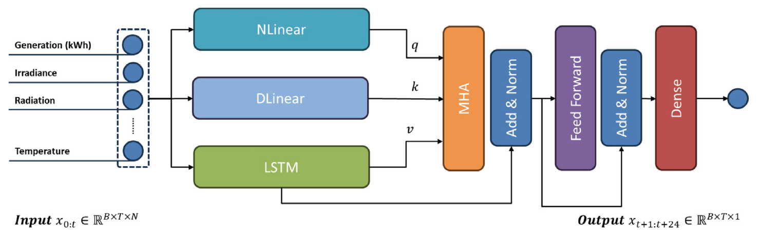
[TeX:] $$W_S \text { and } W_D$$ represent wind speed and wind direction, respectively, and [TeX:] $$T_S$$ is a timestamp representing the time in seconds since 00:00 (UTC) on January 1, 1970. Seconds of the Day ([TeX:] $$SoD$$) is a value representing the time elapsed from midnight to the present time, expressing a day in seconds.

Fig. 5.

Distribution of power generation by time interval

4.2 Hybrid Model Structure

The structure of the hybrid model proposed in this paper is as shown in Fig. 6. In order to accurately perform the challenging task of power generation prediction, we learn sequential features as well as extract and reflect trends and irregular features. The input data [TeX:] $$x_{0: t} \in \mathbb{R}^{B \times T \times N},$$ which consists of N weather data and power generation for T hours with batch size B, is learned and features are extracted using three backbone models: LSTM, DLinear, and NLinear. DLinear learns the trend of the input data and extracts features reflecting it, and NLinear learns differences to learn and extract irregular time series features. LSTM learns sequential features and generates an overall prediction value. Each prediction can be expressed as follows (3):

In addition, to effectively integrate the output of each backbone model, the Multi-Head Attention (MHA) structure is used to distribute it to k parallel heads, each of which performs self-attention tasks. Each head computes a dimension of size [TeX:] $$d_x$$, and MHA can be expressed as follows (4):

The outputs [TeX:] $$O_N \text { and } O_D$$ obtained from NLinear and DLinear generate an attention matrix based on the trend and irregular features of the input data, and are multiplied by the output [TeX:] $$O_L$$ of LSTM to suppress unnecessary features and allow the model to focus on important features.

After that, the attention-reflected features are refined through the Feed Forward Network (FFN) based on Multi Layer Perceptron (MLP), and the last Dense layer compresses the features with the size of N into a single power feature. The final output of the model [TeX:] $$x_{t+1: t+24} \in \mathbb{R}^{B \times T \times 1}$$ can be expressed as follows (5):

The proposed hybrid model can reflect the trend and irregular features captured from linear models in the prediction of LSTM, thereby richly reflecting the features of time series data. In addition, it suppresses unnecessary features by using self-attention technique, and allows the model to focus on important features, enabling robust and accurate prediction.

Fig. 6.

Hybrid model structure

5. Experiments

In order to demonstrate the superiority of the hybrid model proposed in this paper, we conducted comparative experiments with other time series forecasting models. In addition, to ensure the robustness of the experimental results, we conducted a ablation study on the prediction length and the combining method.

5.1 Implementation Details

The experiments were conducted on Python 3.9.13, Tensorflow 2.10.1 and Keras 2.10.0 with Intel(R) Core(TM) i7-10700 CPU @ 2.90GHz, RTX 3070 environment in Windows 10 WSL. The batch size is set to 256, and training is performed with the AdamW optimizer with a learning rate of 0.0005 for 100 iterations and the MSE loss function.

The dataset is configured to predict the future for 24 hours based on 24-hour input data using the sliding window technique [31], and the value range is normalized to 0 to 1 through Min-Max normalization. Of the total 19,680 data, 17,520 data for 2 years are used for training, and the remaining 2,160 data are divided in half and used for validation and testing, respectively.

5.2 Metrics

Evaluation is performed with actual value range by performing denormalization on the predicted values. In addition to Root Mean Squared Error (RMSE) and MAE, mMAPE [32] and R² are also used as metrics to provide more intuitive indicators.

RMSE and MAE represent the difference between the predicted value and the actual value, respectively, and along with mMAPE, the lower the value, the better the prediction quality. mMAPE represents the degree of error in the predicted value as a percentage between 0 and 100. R² represents the maximum explanatory power of the model, and the higher the value, the better the explanatory power. Each metric for the actual value y and the predicted value [TeX:] $$\hat{y}$$ can be expressed as (6):

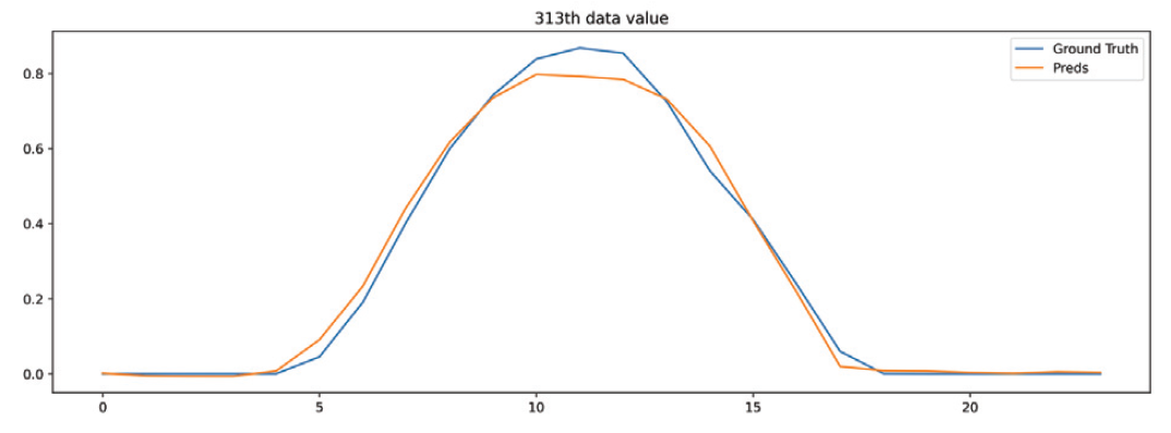
5.3 Experimental Results

The quantitative comparison results with other models measured using test data are shown in Table 1. The comparison results show that the hybrid model proposed in this paper achieved the best results in all four metrics, and showed about 10% improved prediction quality compared to the single-structure model, proving the superiority of the proposed structure.

In addition, as shown in the Fig. 7, the hybrid model’s predicted values and actual values were compared for arbitrary test data, and it was confirmed that it could generate predictions similar to the actual values.

Fig. 7.

Prediction results of the hybrid model

5.4 Ablation Study

Additionally, we conduct ablation studies to test the performance of different concatenation methods for different prediction lengths. Table 2 shows the performance changes by concatenation methods and prediction lengths. The common method of concatenating each output does not significantly improve performance because it does not extract valid features well, and it also increases complexity by doubling the number of dimensions. On the other hand, when concatenating based on self-attention techniques, it shows higher performance than a single model, proving that it is useful to reflect both trends and irregularities using the outputs of three models.

6. Future Work

Future work could be conducted by extending the dataset to also include weather data and power generation data from power plants in other regions, both within Korea and maybe even beyond. The model could be extended to also accept positional information and with that spatially aware DL blocks, so that a single model could be trained to handle all the different locations, therefore training a model that could potently even, to some extend, generalize in a way where it can predict the power for new plants without additional training. Another possible future direction would be the attempt to predict even further into the future, a task that is not trivial by any means. One could, for example, consider utilizing real live weather forecast data to provide the model with more relevant and more reliable weather data for future timesteps, so that the results can be based on those.

7. Conclusion

In this study, we tackled the challenges of forecasting solar power generation, which is critical for the efficient use of renewable energy. We proposed a hybrid model that combines LSTM and linear models with a multi-head attention mechanism. This approach effectively captures both short-term variations and long-term trends in time series data, addressing the inherent unpredictability of renewable energy sources. Our experimental results show that the proposed model outperforms existing prediction models by approximately 10%, achieving an RMSE of 50.68, MAE of 26.12, mMAPE of 6.43, and an R² value of 0.80. These metrics confirm the model's ability to deliver more accurate and reliable solar power forecasts compared to other methods. By improving prediction accuracy, this hybrid approach can enhance the integration of renewable energy into power grids, enabling better energy management and storage planning.